Mark Holcomb owns Dynamic Systems Engineering in Roseville, California, and has been working in the motion space for 30 years, doing structural dynamic testing/modeling and simulation, motion control, sales and product management. He will present “Applied Vibration Theory: A Guide to Vibration Troubleshooting and Measurement Techniques" during A3's Automate Show in Chicago's McCormick Place on May 6 at 2:30 pm. For documents and assistance with calculating FRF and auto spectrum, contact him at [email protected].
Motion systems inherently have a problem that occurs over time. This unavoidable problem is “change.”
System dynamics change with temperature, with cleanliness, with wear and with fatigue. Once any one of these changes reaches a point where the existing dynamics are so different from the initial state, or expected dynamics, the system enters an unknown state of performance, and in the worst-case scenario can fail, often in a catastrophic manner.
The recovery cost of even minor, much less major failures is often measured in thousands, if not tens of thousands of dollars. The lost revenue of a down system will often be an order of magnitude worse than the recovery itself, making this always-lurking issue a huge factor in complex motion systems.
Getting in front of motion system failures, however, is not as difficult as one may think. The solution exists in designing into the machine the right sensors, selecting the right servo drive and creating the needed code to measure and compare data on the fly. This is essentially a frequency fingerprint of the system, capturing its uniqueness and similarity to the fleet. Making machines smarter is the digital transformation that factories will rely on to remain competitive. Hardware and software are needed to execute real-time system dynamics identification, monitoring and decision-making.
In situ sensors
Let’s discuss some of the commonly available sensors often found within motion systems, and how, or if, they can be used to monitor change.
Limit switches are a workhorse sensor in automation. These types of sensors are likely the oldest and most widely used because of their relevance. Their inherent value is their simplicity. The outcome is binary. The answer is either yes or no. At the most fundamental and simplistic level of real-time monitoring is the notion of assessing whether the system is where it is supposed to be. Limit switches can provide this information, but the yes-or-no aspect of the output limits its value, making a second level of information needed.
The servo loop and its most common position sensor, the encoder, is the next step in determining the answer to the question: Is the machine where it is supposed to be? Encoders have almost unlimited resolution capability and can be made with incredible accuracy, defining sub-micron positional knowledge. These sensors, along with Eddy current, linear variable differential transformer (LVDT) and a host of other similar position-sensing technologies, mean, if encoders or similar sensing are being used, we have everything we need, right? The short answer: No, we don’t.
Servo loop sensors are often designed around the motor, with the encoder close by, so the control of motor is as simple and straightforward as possible. Nothing is for free in controls, and the cost of simplicity is paid for in lack of information of the load the servo is moving. The load is often mechanically away from the encoder, separated by bearings and flexible structures that move with temperature and dynamic forces. Sensors such as laser interferometers, or optical focus type sensors, do a great job of measuring the position of the load, so, in part, we are now a step closer to the real-time monitoring of what matters most to the motion system, the position of the load.
Similar to position sensors are a wide variety of servo loop sensors for metrics, such as position error, velocity error, current and current error. These are all very useful metrics and should be part of the real-time fingerprint, as they will be one of the leading indicators of when a problem does arise.
The challenge with these sensors is that they are limited in their reach. If, for instance, the position and current loop error signals have a 30% increase in their root mean square (RMS) value, the root cause is still unknown. Experienced servo engineers would likely look at stability data such as Bode plots gain margin and phase margin, but knowing where to look beyond that is pure guesswork.
If a motion system is experiencing a rise in temperature, for whatever reason, and the stiffness of the system changes in a way such that a resonant frequency changes, maybe away from a fixed notch filter, or low pass filter, such that attenuation is reduced and gain margin becomes marginal, that resonance will now linger in its response to motion. The Bode plot may be able to capture the gain margin issue, but it won’t be able to identify the subsystem that has changed.
Embedded Sensors
Servo sensors for position, velocity, current, error and the like, and load-measuring sensors should always be used in the real-time monitoring system, but they too lack something critical. The missing element is in subsystem knowledge. Subsystem knowledge is a fingerprint of the mechanics making up the motion system. This would be components such as the x stage of a cartesian robot, or the third joint of six-degrees-of-freedom cobot, or maybe the z axis of x-y-z-Theta stage. These subsystems have their own dynamics and as such should be monitored as separate entities so troubleshooting can be very specific to where the problem resides.
The sensor that best enables subsystem testing is an inertial sensor such as an accelerometer or geophone. Accelerometers and geophones have many benefits, including their compact size, lightweight mass, simple signal conditioning and ability to sense sub-micron and nanometer-level vibration across a wide frequency range. Designing these sensors into the fabric of the mechanics will unlock the ability to quickly identify subcomponent performance and get to root cause.
Table 1 illustrates common sensors and their pros and cons. There are many options to pick from, and each has a pro and a con. Overall, when considering all aspects, accelerometers or microphones are often the best choices for embedding motion sensors into the system.
Regarding accelerometers, they come in many shapes, sizes, performance capabilities and of course costs. The low-cost end of the spectrum almost always means poor low frequency response and probably means they are printed circuit board (PCB) compatible. This opens a huge opportunity to undo all of the good that adding an embedded sensor can bring. A PCB accelerometer can be useful if the right design considerations are made, namely the mounting of the chip to the PCB and the PCB to the hardware.
Any amount of compliance, lack of stiffness, means the accelerometer will be responding to its own mounting structure rather than the structure it is intended to measure.
Measurements
Now that we have our embedded accelerometer identified, we need to understand which measurements will best identify how the system has changed. Two types of measurements are needed, the frequency response function (FRF) and a sub-calculation of the FRF, the auto power spectrum (APS).
The FRF is based on one signal’s relationship to another. It is simply an output compared to an input, displayed in magnitude and phase, as a function of frequency. Without going into the detailed mathematics of the fast Fourier transform (FFT), the building block of the FRF, let’s focus on two aspects: how it is constructed and how to interpret the results.

Figure 1 shows the process by which an FRF is calculated. There are two signals, the input, which is commonly force or torque, and output, in our case the accelerometer signal. The recorded signals are windowed and then processed into magnitude and phase versus frequency.

An example outcome is shown in Figure 2. The tall peaks are the system’s resonances, and these are the fingerprint of the subsystem. In the figure, let’s say the original curve was how the substructure presented when it was commissioned, and the modified line is the substructure after and while the system was experiencing an increase in temperature.
As you can see, the resonance near 780 Hz has shifted to below 700 Hz, and right away this substructure would be investigated as to why a major mechanical change was occurring.

A second use case for the FRF is to monitor damping. Damping is related to the amplification factor, or Q factor. A simple and generally accepted method for damping assessment is the formula Q=1/(2*zeta), where zeta is the damping ratio defined in the simple spring-mass-damper model of mx’’(t) + cx’(t) + kx(t) = f(t), normalized to X’’ + 2*zeta*w X’ + w2 = f(t), where c = 2*zeta*w*m and k= w2*m. This approximation is useful for widely separated resonances, where each can be treated as a single degree-of-freedom (DOF) system. A more accurate method when there are many closely spaced resonances is to use a 3 dB band calculation to get to the Q value (Figure 3). In this case, Q = f0/BW, and BW = f2 - f1.

Zeta is often stated as a percent, meaning 1% zeta is a value of 0.01. Aluminum structures will generally have 0.1-0.2% zeta damping. Figure 4 is a real-life example of a shift in structure damping at 113 Hz. Substructure FRF data can identify these types of system changes, and, with proper specification, any shift would be captured immediately, reducing the potential for exponential loss in the form of damaged parts and system troubleshooting.
One challenge with FRF data is that the system cannot be running in normal operational mode when data is being collected. The machine must be stopped while the servo drive injects force or torque into the system. The good news is that measurements should only take a few minutes each, and the system, provided everything passes, can proceed to normal operation within minutes. This diagnostic could be programmed to run once daily, weekly or monthly, all based on the risk and normal maintenance schedule.
Unlike the FRF, the APS measurement is only of one signal and does not need the system to come out of normal operational mode. In fact, these measurements are most useful when collected during normal operation, to capture any change while it is occurring.
Like the FRF, the APS is an outcome of the FFT, meaning the signal is windowed first and then the FFT is calculated on the windowed data. We will not go into the specifics of the many window options, only to say the Hanning window is the best and most common option.

The basic premise of this data is to have a frequency-based signature of each major subcomponent, based on real-time movement of the system. As the system starts experiencing change of some form, the resonances of the system may change (Figure 5) in frequency, damping, or both, and the APS plot will capture this effect. Other changes could be that a band of energy, not just a single resonance may increase (Figure 6.). Figure 5 is an example of auto spectrums of passing and failing data collected with an accelerometer during tool operation.

Regarding auto power and auto spectrums, there are two options regarding how the data is displayed. The power spectrum is best used when the end goal is either to overlay signals taken with different sample rates or to ultimately integrate the frequency data to get to an RMS value.
The power spectrum is unique, in that each magnitude on each frequency band is normalized to the frequency width. This makes data in some ways universal, which is a valuable feature. The downside is that the amplitude at each spectral line is not the actual amplitude, but, if integrated across a band, the RMS is preserved.
The auto spectrum, however, is not normalized to the frequency band but does represent the amplitude of the peak correctly. Signal-processing engineers have no shortage of strong opinions on this topic, but, in my experience, when measuring mixed signals, meaning those containing broad band noise, single tones and resonant content, it is best to use the auto spectrum with a frequency as close to 1 Hz as possible. This opinion is based mostly on the fact we most often deal with resonant or forced response peaks and rarely with the energy across a band.
A critical part of executing the APS measurement is to always collect the data under the same environmental variables. Any change in the operation of the machine while data is being collected will change the outcome. Since the data will be collected by the servo drive, synchronizing a repeatable test during a known state of the machine should not be an issue.
Data may be desirable under multiple modes of operation, such as a constant speed or just after moving and settling. Steady-state vibration collection gives a result that is often influenced by reciprocating motion, such as a bad ball bearing within a race, a mass imbalance, a pump or oscillatory machinery onboard or somewhere within the environment or an audible tone from a wearing part. Transient vibration, by definition, is only present for a short period of time, so capturing it can be challenging. Since the servo drive will be regulating data collection, the drive can trigger data collection at the end of the move trajectory, thereby capturing a few hundred milliseconds of transient vibration data. Transient data is best used to identify any shift in frequency or damping of structure resonances. In both cases, windowing will be needed, and, in the case of transient data collection, care must be taken to trigger the data collection appropriately to not attenuate transient vibration by the window itself. This can be accomplished through pre-triggering, thereby centering and aligning the end of the move with the center of the window.
As mentioned previously, the servo drive is the best choice for executing the FRF and auto spectrum data collection. To be successful, however, the drive must have two analog inputs and the ability to synchronously sample both channels faster than 2.5 kHz. Synchronous sampling is a requirement for the FRF, although if the lag between channels is not significant and the phase information is not used, the synchronous requirement could be relaxed. With a 2.5 kHz sample rate or higher, the usable frequency band of the FRF and auto spectrum is 1,000 Hz, which should be sufficient for most cases.
Embedding more than two sensors is the goal of this approach, so depending on the capabilities of the drive, a secondary digitally controlled multiplexer could be implemented to route the signals to the drive in groups of two, four, six or eight, depending on the number of available analog inputs.
There are many accelerometers readily available to serve machine builders’ needs, from stand-alone, threaded mount options to PCB chip-based packages. Mass and size should be weighed against performance requirements, including shock loads, vibration range and temperature sensitivity.
Most accelerometers will need an integrated-circuit-piezoelectric (ICP) charge converter to change output to +/-10 V. The ICP circuit can be purchased as a stand-alone device, or it can be easily constructed as a daughter board to the servo drive or multiplexer.
Cabling can influence the structure by limiting its travel or by adding stiffness and damping. There are many choices when choosing accelerometers, and each comes with an assortment of cabling options. Pick the one that meets your needs. Be sure to consider length, flexibility, fatigue and shielding when making your choice.
For the FRF data, the system will need a force or torque input. Since the machine is likely to have no shortage of linear, rotary or rotary-to-linear actuators and motors, using these are the best approach.
Servo-drive manufactures likely already have the FRF and subsequent auto spectrum and windowing algorithm as part of their Bode plot capabilities. If they do not, you may want to upgrade your choice of servo drives, as the Bode utility is an excellent tool for control loop tuning and stability assessment. If they do not and you have no other choice but to use the existing drive, you will need them to embed the calculations into their firmware or, at a minimum, record the data and upload it to a controller with the capability or export the data to a host PC. If exporting is the only option, the real-time option is now not available.
The FFT is a commonly known calculation and is part of most C, C++ and Python or equivalent coding languages. The trick is not in simply doing the FFT, but in getting the FFT into the auto spectrum and FRF correctly.
There are factors of two and square root of two, in many places within the FRF and auto spectrum calculations, so getting the math correct is essential.
One key step within FRF and auto-spectrum data collection is the notion of averaging. At a minimum, auto-spectrum and FRF data should always be averaged. Averaging reduces errors in the data and provides a statistically more accurate frequency domain representation of the time data. Many advise 30 averages, and I recommend at least 10.
The final capability needed within the software realm is the ability to generate white noise or a swept sine input. Again, this capability is within the Bode plot feature, so if the servo drive is doing Bode plots, it already can generate the signal needed. If it does not, however, white noise and swept sine code is easily found within C, C++, Python and other scripting languages.

Figure 7 shows a simplified block diagram of where the input force/torque should be added into the motor control. In most cases, the servo loop should remain closed, and the disturbance added into the loop, right before the axis command is split into the three motor phases. In the diagram, the white noise/swept sine is shown as an input, but this signal is internally generated within the microprocessor, and not taken in from the outside.
Data analysis and decision making
With hardware and software identified, the final step is creating a decision-making algorithm that deciphers failing from passing. Earlier, I mentioned the use of servo sensors such as position error, velocity error and current loop error as all part of ongoing monitoring. These metrics are always part of servo drives’ embedded fault protection, so there’s no need to discuss any strategies in how to make decisions on real-time servo data. Instead, we need to develop a method of decision making for FRF and APS data, each having at least two degrees of freedom, meaning a magnitude at a frequency repeated many times.
The fundamental aspects of the FRF are the frequency of the resonance and the amplitude. In an ideal case, each subsystem test would be searching for one resonance, but this is likely not going to be common, and each test will be looking at multiple frequencies.
First, the statistical mean of each frequency and each magnitude must be found. This is best found by testing a minimum of three, and preferably 10, systems. For each FRF, the frequencies and amplitudes of each critical resonance are recorded and stored in a lookup table within the servo drive’s random-access memory (RAM).

An error band is needed around each value, something like +/-5% on frequency and +/-10% on amplitude (Figure 8).
The trick to the algorithms will be searching out the peak and tagging the maximum value.
For the amplitude of the resonance, converting the peak using the -3 dB width mentioned previously should be considered as it gives a numerical assignment of damping versus just an amplitude value.
APS data is different than FRF data, in that we are looking for anything out of the ordinary, while also looking for what we expect to see. Accelerometer data is often converted to position, integrated two times. This creates a left-to-right downward slope to the data. The pass-fail criteria is now frequency-dependent and probably different band-to-band throughout the entire range.

Benefits
Although embedding sensors to enable real-time digital fingerprinting of subsystems comes at cost, that cost is quickly recovered in one single prevented failure or one instance of fast-tracking a root cause analysis. The value of having sensors reporting status automatically on set time intervals or at the touch of a button, saves time and resources and enhances team and machine productivity for factory or plant customers.
The ability to remotely access and diagnose machine health benefits the end user in the maintenance scheduling and uptime metrics, and it benefits the machine builder in the value and capability the band creates.
Having the foresight to embed diagnostic capabilities into complex machines involving moving parts that are subject to changes in temperature, wear and environment is an approach that elevates machine-building. Embedded sensors not only help in maintenance and fast-tracking root cause analysis, but they also provide the builder with real-life data of how bearings, motors, gears, belts and pneumatics perform over time.
Knowing the limits of motion components such as motors, bearings, gears, belts, rollers and tensioners, for example, enables the builder to make better choices in design and in accessing the required maintenance for the end user. If the machine builder has data supporting longer service intervals versus a competitor, its factory or plant end user’s uptime will be longer, thus enhancing the machine’s value as a whole.
Conclusion
Industry 4.0 has been discussed for many years, and, in some manufacturing spaces, it is being fully realized. In many others, however, the technology available has yet to be fully realized for many reasons.
With advent of easily accessible and enormously powerful servo-drive capability and algorithm solutions being available across many coding platforms, there is little to no headwind in embracing the introduction of a higher level of subsystem level diagnostics.
The frequency response function and the auto spectrum have been the workhorse tools for vibration analysis for the past 40 years, since the digital FFT was implemented, and should now be a part of every servo drive in the market. Strategic placement of the right sensors within the subsystem and intelligent firmware changes that synchronize data collection with machine activity will create enormous value in predicting maintenance and increasing machine productivity.
With the right specifications and data collection methods, the real-time diagnostic/health-monitoring capability is practically limitless.